The first 5mins with survey data

Step 1: Read the data in with readr

Load up the {tidyverse} and {janitor} for wrangling the dataset into something tidy.

library("tidyverse")
library("janitor")

Read in the data using read_csv() and print thw resulting tibble() to the console… this dataset has 355 rows so I’ve cheated in the blogpost by only showing the first 5 rows

raw_kaggle_survey <- read_csv("data-raw/kaggle_survey_2020_responses.csv")
raw_kaggle_survey %>% 
  select(1:5)

## # A tibble: 20,037 x 5
##    `Time from Start to … Q1         Q2          Q3           Q4                 
##    <chr>                 <chr>      <chr>       <chr>        <chr>              
##  1 Duration (in seconds) What is y… What is yo… In which co… What is the highes…
##  2 1838                  35-39      Man         Colombia     Doctoral degree    
##  3 289287                30-34      Man         United Stat… Master’s degree    
##  4 860                   35-39      Man         Argentina    Bachelor’s degree  
##  5 507                   30-34      Man         United Stat… Master’s degree    
##  6 78                    30-34      Man         Japan        Master’s degree    
##  7 401                   30-34      Man         India        Bachelor’s degree  
##  8 748                   22-24      Man         Brazil       Bachelor’s degree  
##  9 171196                25-29      Woman       China        Master’s degree    
## 10 762                   35-39      Man         Germany      Doctoral degree    
## # … with 20,027 more rows

Step 2: Look for where the question ids and text are kept

Around 90% of the time the following things are true:

• The first few columns contain info about the survey respondent, eg how long they took to answer the survey and if they completed the survey.

• The column names are question ids and the first row contains the actual question text.

Let’s create ourselves a question_index that contains the question_id and the question_text:

question_index <- raw_kaggle_survey %>% 
  slice(1) %>% 
  select(2:ncol(.)) %>% 
  pivot_longer(cols = everything()) %>% 
  rename(question_id = name,
         question_text = value)

Now we can throw out the survey respondent information and the question text by combining slice() and select(), note that you’ll need to throw away different amounts of rows/columns for each survey dataset:

kaggle_survey_2020 <- raw_kaggle_survey %>% 
  select(2:ncol(.)) %>% 
  slice(2:nrow(.))

Step 3: Clean up those question ids

I ensured to load up the {janitor} package at the beginning because I want to ensure the question_ids are standardised. I’ve extracted some example columns where there’s idiosyncratic capitalisation which will likely cause code errors:

kaggle_survey_2020 %>% 
  select(6:10)

## # A tibble: 20,036 x 5
##    Q6          Q7_Part_1 Q7_Part_2 Q7_Part_3 Q7_Part_4
##    <chr>       <chr>     <chr>     <chr>     <chr>    
##  1 5-10 years  Python    R         SQL       C        
##  2 5-10 years  Python    R         SQL       <NA>     
##  3 10-20 years <NA>      <NA>      <NA>      <NA>     
##  4 5-10 years  Python    <NA>      SQL       <NA>     
##  5 3-5 years   Python    <NA>      <NA>      <NA>     
##  6 < 1 years   Python    R         <NA>      <NA>     
##  7 3-5 years   Python    R         <NA>      C        
##  8 < 1 years   <NA>      R         <NA>      <NA>     
##  9 5-10 years  Python    <NA>      SQL       <NA>     
## 10 < 1 years   Python    <NA>      SQL       <NA>     
## # … with 20,026 more rows

All we need to clean the survey data is to use clean_names()

kaggle_survey_2020 <- kaggle_survey_2020 %>% 
  clean_names()
kaggle_survey_2020 %>% 
  select(6:10)

## # A tibble: 20,036 x 5
##    q6          q7_part_1 q7_part_2 q7_part_3 q7_part_4
##    <chr>       <chr>     <chr>     <chr>     <chr>    
##  1 5-10 years  Python    R         SQL       C        
##  2 5-10 years  Python    R         SQL       <NA>     
##  3 10-20 years <NA>      <NA>      <NA>      <NA>     
##  4 5-10 years  Python    <NA>      SQL       <NA>     
##  5 3-5 years   Python    <NA>      <NA>      <NA>     
##  6 < 1 years   Python    R         <NA>      <NA>     
##  7 3-5 years   Python    R         <NA>      C        
##  8 < 1 years   <NA>      R         <NA>      <NA>     
##  9 5-10 years  Python    <NA>      SQL       <NA>     
## 10 < 1 years   Python    <NA>      SQL       <NA>     
## # … with 20,026 more rows

But there’s a nitpicky step of my workflow I need to remember. The question_index dataset needs to be manually updated with make_clean_names().

question_index <- question_index %>% 
  mutate(question_id = make_clean_names(question_id))

I’ve taken to using this workflow after working with a variety of survey datasets where there was additional manual wrangling that needed to be done within these 3 steps.

Step 4: Give {readr} another change to parse the column types

The {readr} does a really good job of guessing column types, except in raw surevey datasets. That’s because the first row usually contains question text which throws off the parser. Forunately, we can give it another go as follows:

kaggle_survey_2020 <- kaggle_survey_2020 %>% 
  type_convert()

… unfortunately, this is one dataset where all question responses truly are characters (or strings). For instance, the respondent age is stored as an age range instead of a specific number.

Exploratory Data Analysis

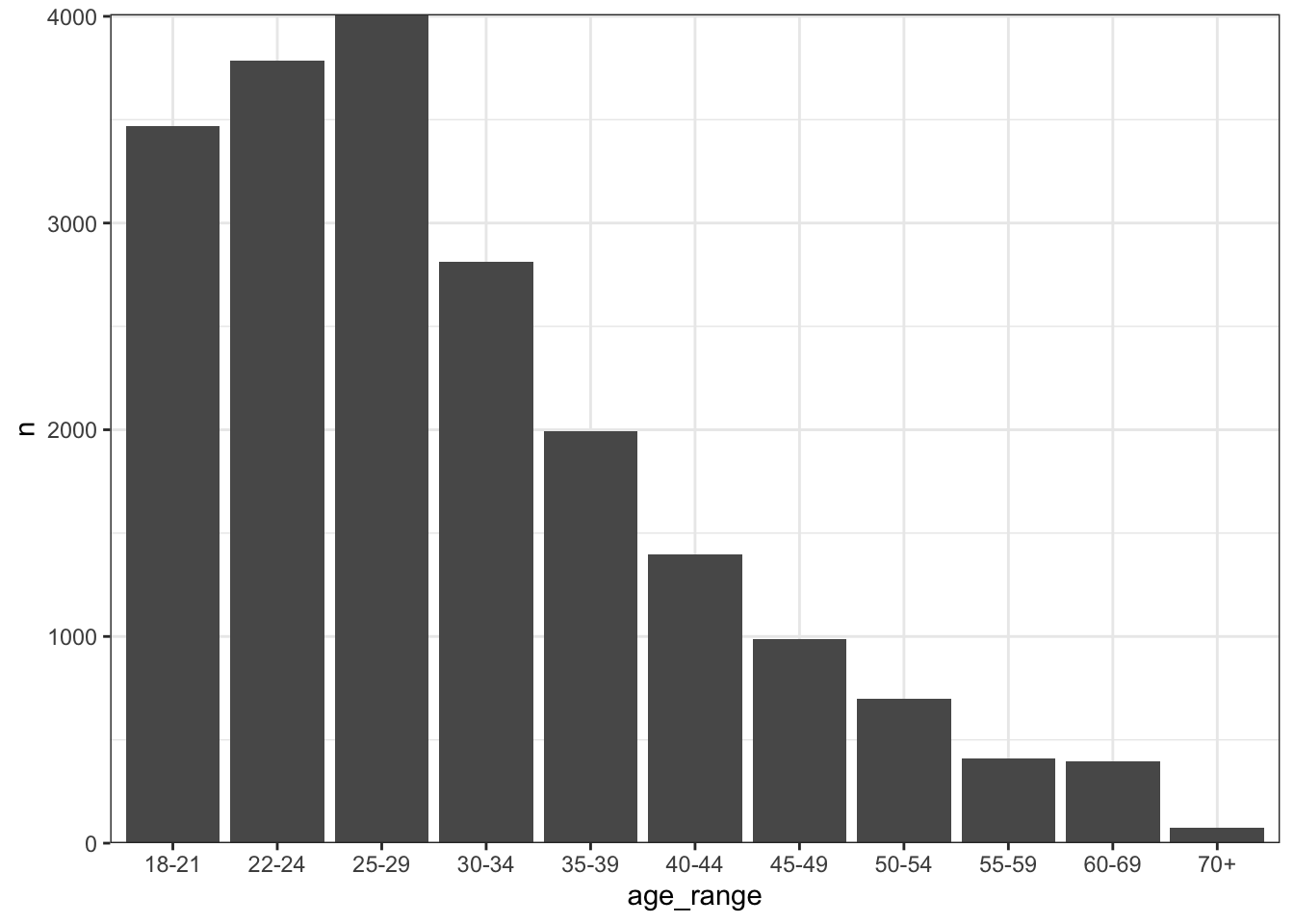
It’s now time to start to explore the survey data, and that’s often going to involve cross-tabulating question responses. I’m going to tag on the recipe that I use for processing age range columns:

kaggle_survey_2020 %>% 
  select(q1) %>% 
  count(q1) %>% 
  rename(age_range = q1) %>% 
  separate(col = age_range,
           into = c("lower_age", "upper_age"),
           remove = FALSE) %>% 
  mutate(age_range = fct_reorder(age_range, lower_age)) %>% 
  ggplot(aes(y = n,
             x = age_range)) +
  geom_col() +
  theme_bw() +
  scale_y_continuous(expand = expansion(add = 0))